I had some trouble developing this component of analysis. As I mentioned in my previous article on four factor offensive efficiency, some things don’t quite translate for defence.
The first and most obvious element for anyone familiar with the sport is that there aren’t clear defensive partners for each offensive statistical category. For example, the opposite of a bucket at the rim in basketball might be a block, but AFL doesn’t really have ‘blocks’ as a defensive measure of denying a score.
We can take into consideration smothers, usually rolled into the measure ‘1 per centers’ on public stats sites, with spoils and other discrete defensive actions. However, smothers are relatively rare and also don’t apply solely to players taking a shot. To this end measuring defence in a quantitative manner is a trickier task.
Because I was basing my approach on Dean Oliver’s four factors for basketball my initial instinct was to simply try and find the reverse factors on defence. Where Oliver’s talking about offensive rebounding rate, for defence he can look at defensive rebounding rate.
The other factors more or less take into consideration the opponents results on offence. For example, in defensive four factors Oliver would look at the opponent’s effective field goal rate as the corollary to your own effective field goal percentage. We can do this too when we’re looking at team data.
In that case we would look at the defensive four factors as:
- opponent effective scoring rate;
- opponent advancement rate;
- opponent turnover ration; and
- opponent offensive retention.
This works just fine if you’re looking at team data where we only need to apply the data to the whole unit, but if we want some individual results, we have a different problem. For example, there is no ‘metres restricted’ or ‘metres decreased’ as a specific individual measure for a player’s defence. Additionally what we are really doing here is just comparing one team’s average offence versus the average offence they allow. It’s bot a bad measure of defensive prowess, but (a) I don’t know if this tells the whole story and (b) it cannot be applied to individual stats to get a quantitative figure for defence.
If we take a look at this initial approach, we can see that the top three teams in 2018 for defensive efficiency were Richmond, Geelong and Hawthorn. This is a somewhat interesting result. Both Richmond and Geelong were in the top three for least points conceded, so their defensive efficiency status might come as little surprise.
Hawthorn, on the other hand, actually ranked eighth for points conceded but were third by my measure of defensive efficiency. This perhaps speaks to the fact that relative to game speed and volume of possession the Hawks defence is arguably still quite good. And although we are only talking about small differences between actual points and predicted points we can also see that not much separates teams.
| Team
| Opp EffScRate |
Opp TO Rate |
Opp MetresG |
Opp Off Ret |
Actual |
Predicted |
| Tigers |
0.342 |
0.155 |
0.057 |
0.98 |
72.5 |
71.4 |
| Cats |
0.340 |
0.157 |
0.057 |
1.05 |
70.7 |
73.0 |
| Hawks |
8.000 |
6.000 |
1.000 |
1.00 |
76.5 |
74.0 |
| Magpies |
0.363 |
0.160 |
0.056 |
1.01 |
76.3 |
74.8 |
| Giants |
0.346 |
0.146 |
0.058 |
1.06 |
73.3 |
75.7 |
| Power |
0.358 |
0.161 |
0.057 |
1.06 |
74.8 |
75.8 |
| Eagles |
0.361 |
0.156 |
0.057 |
1.04 |
74.4 |
76.1 |
| Swans |
0.357 |
0.154 |
0.055 |
1.12 |
75.9 |
77.3 |
| Demons |
0.390 |
0.150 |
0.056 |
0.97 |
79.5 |
78.9 |
| Kangaroos |
0.381 |
0.155 |
0.055 |
1.07 |
81.6 |
79.8 |
| Bombers |
0.403 |
0.138 |
0.056 |
1.05 |
83.5 |
84.1 |
| Crows |
0.395 |
0.148 |
0.059 |
1.06 |
84.9 |
84.3 |
| Dockers |
0.418 |
0.144 |
0.058 |
1.12 |
92.9 |
89.9 |
| Bulldogs |
0.429 |
0.147 |
0.057 |
1.11 |
92.4 |
90.6 |
| Lions |
0.446 |
0.145 |
0.056 |
1.12 |
93.1 |
93.7 |
| Saints |
0.448 |
0.133 |
0.057 |
1.11 |
96.6 |
94.9 |
| Suns |
0.428 |
0.141 |
0.062 |
1.23 |
99 |
97.4 |
| Blues |
0.477 |
0.140 |
0.057 |
1.14 |
103.5 |
100.4 |
Continuing with Hawthorn as the example, an improvement of only one less goal conceded per game would make them the best defence in the game. Using my defensive efficiency formula Hawthorn could achieve this is by tweaking only a few aspects of their play.
In regard to the four factors the Hawks rank as the No. 1 team in opposition offensive retention and opposition advancement rate, meaning they are good at restricting the opposition’s run and perhaps long kicking and also don’t allow the opposition to hold the ball in their own forward half for very long. In the other two categories they rank sixth for opposition turnover rate and eighth for opposition effective scoring.
Looking at these two areas for improvement, we could posit Hawthorn turning one opposition goal from last season into a behind this season and forcing one extra error out of the opposition each game for 22 more total forced errors on the season. These seemingly small improvements would take Hawthorn’s predicted score against to a little over 65 points per game which, if realised, in actuality would be the most miserly offence in some time.
Indeed to put it in perspective only three teams have averaged fewer than 65 points per game since the 1967 season.
| Season |
Team |
Ave points against |
| 2009 |
Saints |
64.13 |
| 1968 |
Saints |
63.15 |
| 1967 |
Blues |
62.9 |
Obviously this is easier imagined by my model than done in reality, but I think this gives a feel for how small changes in on-field actions adjust the bottom line.
So more or less I like looking at defence for teams using this model. It runs pretty close to actual results and makes good sense. However, it’s not great for the individual defence, and this is where my analysis becomes more complex and probably less reliable.
First of all, when doing big data set analysis of typical defensive indicators I found that there is little or indeed opposite correlation with being scored against. That is, if we look at, say, the numbers of spoils or rebound 50s as it relates to being scored against, we actually find that more rebound 50s happen in losing teams that do get scored against. What we would be hoping for is that more defensive stats correlate with restricting opposition scoring.
Even when we look at those metrics relative to opposition 50s, which might account for the players who are doing the best or most defending relative to the amount of pressure they’re under, also does not show a strong relationship.
It’s although worth mentioning that the difference in what we are trying to achieve with the defensive metric is the inverse relationship to our offensive factors. In other words, when a player does defensive things it reduces their cost on defence. What this means is we are basically saying that if every team gets scored against, every player is to varying degrees responsible for this and as such their ‘defensive cost’ is better if it is lower.
What I found was that the things players do that correlate strongly with lower opposition scores are:
- contested possession;
- kicking;
- metres gained; and
- intercept marking.
I felt there was some difficulty in just building out a model with these stats alone. Ultimately this would probably overrate contested possession midfielders as the best defenders on the ground. Although I think there’s something in that, the point of what this model is supposed to achieve is a reflection of defensive efficiency, primarily by those players who are mostly engaged with the job of actually defending.
In the end what I have tried to produce is a model with correlation and relevance so that it is predictive of the actual score, albeit not as strong as with the offensive model, but which also reflects legitimate defensive actions.
What I attempted to develop was:
- defensive release, an attempt to reflect the opposite of offensive retention; and
- effective ‘stop’ rate, an attempt to reflect the opposite of effective scoring rate
Ultimately, however, I found that trying to have separate metrics to build a similar multivariable linear model as with the offensive efficiency simply never gave a result that was reliable enough to keep me happy. What I’ve ended up with is a single metric combined of the following stats which I think still gets at the notion of ‘stopping’ and ‘releasing’ from defence:
- kicking;
- rebound 50;
- contested possession;
- 1 per centers (spoils, smothers, knock-ons);
- intercept marks;
- minus marks inside 50; and
- minus tackles inside 50
All of this smushed together and then divided by the number of opposition entries inside 50 gave a very strong correlation to not being scored against. Indeed I was happy enough with the pattern this metric created with opposition scoring to build an exponential regression model as opposed to a linear one.
I might be stretching a tiny bit with the exponential relationship, but the linear model had about as much error as the exponential one and I like the idea that the model creates a bit more separation between points than a linear model does.
Ranking team defence with my new metric gives the following results.
| Team |
K |
D |
Opp In50 |
T |
R50 |
CP |
MI5 |
0.01 |
ITC |
T50 |
Def metric |
Predicted |
Actual |
| Demons |
209.6 |
386.2 |
55.4 |
69.2 |
33 |
160 |
14.6 |
46.8 |
75.7 |
12.4 |
11.94316 |
72.1 |
79.5 |
| Hawks |
218.9 |
376.5 |
51.7 |
68.9 |
30.8 |
142.5 |
11.8 |
56.6 |
72.9 |
12.7 |
11.94304 |
72.1 |
76.5 |
| Tigers |
207.2 |
366.8 |
54 |
62.4 |
34.8 |
148 |
13 |
54.9 |
83 |
12.1 |
11.58197 |
75.6 |
72.5 |
| Magpies |
217.6 |
399.1 |
52 |
68.3 |
35.8 |
152.5 |
11.2 |
52.2 |
75.2 |
10 |
11.56175 |
75.8 |
76.3 |
| Power |
219.6 |
375.6 |
52.4 |
70 |
38.9 |
149.4 |
11.2 |
60.8 |
73.8 |
12.7 |
11.19011 |
79.6 |
74.8 |
| Crows |
223.6 |
382.9 |
47.5 |
64.6 |
36.7 |
153.6 |
9.4 |
47.2 |
77 |
11.4 |
11.10496 |
80.5 |
84.9 |
| Eagles |
227.2 |
356 |
54.8 |
61 |
36.7 |
143.8 |
11.6 |
49.6 |
72.2 |
10.7 |
11.09766 |
80.6 |
74.4 |
| Giants |
219 |
377.9 |
51.2 |
67.2 |
39.9 |
149.7 |
10.6 |
54.7 |
73.8 |
11.6 |
10.98302 |
81.8 |
73.3 |
| Cats |
210.1 |
380.8 |
53 |
66.9 |
38 |
150 |
12 |
50.5 |
70.7 |
11.3 |
10.825 |
83.5 |
70.7 |
| Bombers |
217.7 |
381.6 |
47.4 |
66.7 |
36.8 |
143.4 |
12.2 |
47.5 |
70.3 |
11.8 |
10.80077 |
83.8 |
83.5 |
| Kangaroos |
201.4 |
367.8 |
52.7 |
62.4 |
35.1 |
148.6 |
11.3 |
44.1 |
74.8 |
10.2 |
10.33966 |
89.0 |
81.6 |
| Swans |
210.7 |
371.6 |
55.2 |
64.8 |
43.2 |
147 |
10.3 |
46.6 |
71 |
9.9 |
10.1277 |
91.5 |
75.9 |
| Bulldogs |
207.5 |
387.6 |
50.2 |
63 |
36.3 |
139.4 |
11.3 |
51.6 |
71.8 |
11.7 |
10.12222 |
91.6 |
92.4 |
| Saints |
207.3 |
388.7 |
52.6 |
60 |
35.4 |
135.6 |
10.7 |
48.1 |
68.7 |
9.4 |
9.925788 |
94.0 |
96.6 |
| Lions |
215.1 |
373.4 |
53.9 |
58.2 |
38.1 |
136.2 |
11.9 |
51.6 |
65.5 |
9.9 |
9.835145 |
95.1 |
93.1 |
| Dockers |
202.9 |
363.1 |
60.7 |
60.2 |
37.5 |
135.9 |
9.9 |
47.2 |
68.2 |
8.1 |
9.742701 |
96.3 |
92.9 |
| Blues |
202.9 |
347.1 |
55.6 |
63.4 |
36 |
135.6 |
9.2 |
48.1 |
63 |
8.4 |
9.592058 |
98.2 |
103.5 |
| Suns |
202.7 |
339.8 |
48.8 |
69.3 |
43 |
144.1 |
7.5 |
52.2 |
71.6 |
11.9 |
9.283361 |
102.3 |
99 |
We see, for example, that Hawthorn and Richmond remain in the top three in terms of efficiency but Melbourne shoot to the first spot in the rankings and Geelong slide way down to ninth spot. In that case, although Geelong conceded only 70.7 points per game, this measure suggests their defensive efficiency is closer to 83.5 points per game.
Going back to the example of last year’s grand final, we can now apply individual defensive scores to each player and maybe establish a more well-rounded picture of performance on the day.
| Player |
Team |
K |
HB |
D |
Def Metric |
Pred Def |
Pred Off |
Net |
| Luke Shuey |
WC |
21 |
13 |
34 |
27.50 |
0.43 |
7.92 |
7.5 |
| Jordan de Goey |
Coll |
12 |
1 |
13 |
7.68 |
5.74 |
12.50 |
6.8 |
| Joshua Kennedy |
WC |
14 |
4 |
18 |
7.79 |
5.65 |
12.35 |
6.7 |
| Mason Cox |
Coll |
9 |
0 |
9 |
8.38 |
5.23 |
10.07 |
4.8 |
| Willie Rioli |
WC |
5 |
7 |
12 |
9.17 |
4.72 |
9.43 |
4.7 |
| Jaidyn Stephenson |
Coll |
6 |
3 |
9 |
3.84 |
9.49 |
13.82 |
4.3 |
| Dominic Sheed |
WC |
17 |
15 |
32 |
17.42 |
1.60 |
5.77 |
4.2 |
| Taylor Adams |
Coll |
22 |
9 |
31 |
18.51 |
1.39 |
5.50 |
4.1 |
| Elliot Yeo |
WC |
12 |
7 |
19 |
18.33 |
1.42 |
4.83 |
3.4 |
| Travis Varcoe |
Coll |
8 |
3 |
11 |
9.08 |
4.77 |
8.01 |
3.2 |
| Brody Mihocek |
Coll |
10 |
5 |
15 |
7.68 |
5.74 |
7.76 |
2.0 |
| Nathan Vardy |
WC |
7 |
7 |
14 |
9.63 |
4.44 |
6.27 |
1.8 |
| Jamie Cripps |
WC |
10 |
6 |
16 |
9.63 |
4.44 |
6.07 |
1.6 |
| Jack Crisp |
Coll |
18 |
7 |
25 |
15.71 |
2.00 |
2.99 |
1.0 |
| Tom Barrass |
WC |
15 |
2 |
17 |
21.08 |
0.99 |
1.55 |
0.6 |
| Jack Darling |
WC |
8 |
4 |
12 |
9.17 |
4.72 |
5.25 |
0.5 |
| Mark Hutchings |
WC |
11 |
4 |
15 |
11.46 |
3.49 |
3.92 |
0.4 |
| Shannon Hurn |
WC |
16 |
5 |
21 |
16.50 |
1.80 |
2.13 |
0.3 |
| Adam Treloar |
Coll |
12 |
14 |
26 |
13.97 |
2.51 |
2.47 |
0.0 |
| Tom Langdon |
Coll |
10 |
13 |
23 |
16.41 |
1.82 |
1.43 |
-0.4 |
| Jack Redden |
WC |
15 |
6 |
21 |
16.96 |
1.70 |
1.08 |
-0.6 |
| Tom Phillips |
Coll |
15 |
6 |
21 |
12.22 |
3.16 |
2.52 |
-0.6 |
| Will H-Elliott |
Coll |
13 |
5 |
18 |
6.98 |
6.29 |
5.64 |
-0.6 |
| Jeremy McGovern |
WC |
12 |
2 |
14 |
19.25 |
1.26 |
0.35 |
-0.9 |
| Jeremy Howe |
Coll |
12 |
1 |
13 |
15.02 |
2.19 |
1.23 |
-1.0 |
| Liam Duggan |
WC |
10 |
6 |
16 |
10.54 |
3.94 |
1.95 |
-2.0 |
| Christopher Mayne |
Coll |
7 |
8 |
15 |
12.92 |
2.88 |
0.50 |
-2.4 |
| Tom Cole |
WC |
8 |
5 |
13 |
11.92 |
3.29 |
0.79 |
-2.5 |
| Brayden Sier |
Coll |
9 |
12 |
21 |
11.87 |
3.31 |
0.32 |
-3.0 |
| Josh Thomas |
Coll |
6 |
7 |
13 |
6.98 |
6.29 |
3.07 |
-3.2 |
| Will Schofield |
WC |
7 |
2 |
9 |
13.75 |
2.59 |
-0.78 |
-3.4 |
| Lewis Jetta |
WC |
9 |
4 |
13 |
9.17 |
4.72 |
1.30 |
-3.4 |
| Liam Ryan |
WC |
6 |
4 |
10 |
6.42 |
6.77 |
3.21 |
-3.6 |
| Scott Lycett |
WC |
4 |
5 |
9 |
7.79 |
5.65 |
1.92 |
-3.7 |
| Chris Masten |
WC |
8 |
6 |
14 |
8.25 |
5.32 |
1.40 |
-3.9 |
| Scott Pendlebury |
Coll |
9 |
11 |
20 |
11.17 |
3.63 |
-0.70 |
-4.3 |
| Mark Lecras |
WC |
5 |
5 |
10 |
7.33 |
6.00 |
1.29 |
-4.7 |
| Brayden Maynard |
Coll |
7 |
2 |
9 |
7.68 |
5.74 |
0.80 |
-4.9 |
| Brodie Grundy |
Coll |
5 |
5 |
10 |
6.98 |
6.29 |
0.04 |
-6.2 |
| Steele Sidebottom |
Coll |
7 |
7 |
14 |
6.98 |
6.29 |
-0.42 |
-6.7 |
| Tyson Goldsack |
Coll |
1 |
8 |
9 |
8.38 |
5.23 |
-1.60 |
-6.8 |
| James Aish |
Coll |
5 |
2 |
7 |
6.63 |
6.58 |
-0.50 |
-7.1 |
| Levi Greenwood |
Coll |
4 |
4 |
8 |
4.19 |
9.07 |
-1.59 |
-10.7 |
| Daniel Venables |
WC |
1 |
3 |
4 |
4.58 |
8.61 |
-2.60 |
-11.2 |
As a test case I’m happy that this metric establishes a realistic but also an interesting explanation of efficiency and performance. To begin with, we can see that the least cost or best defensive players on the day were Luke Shuey, Tom Barrass and Jeremy McGovern. I think this fits with a subjective ‘eye-test’ and also makes some sense in respect to how we know the game is played and where defence comes from.
Especially pleasing from my point of view is that when I combined offensive efficiency with defensive efficiency to produce net results a sensible albeit interesting picture starts to emerge in terms of performance. The best player in the game comes out as Luke Shuey, which, to be honest, had my results produced anything other than Shuey as the top player, I would’ve felt that the model was fundamentally broken.
Following Shuey are Jordan DeGoey and Josh Kennedy – not unreasonable estimates for second and third best but also interesting insofar as both players touched the ball only 13 and 18 times respectively.
Another area I’d like to explore more is the concept of ‘threshold’ wins and losses. With more analysis we can get a measure for an average or replacement-level player. I still don’t have that, yet I can say that the average player in this game was worth -0.9 of a point. Given this we can estimate the player’s impact on the end result by asking what the score would have been if this player was replaced with an average replacement. By that measure we can say if the following West Coast players were replaced by a game average player in a game decided by five points, West Coast would have lost without them:
- Luke Shuey
- Josh Kennedy
- Willie Rioli
- Dom Sheed
On the flip side, in a loss of five points the following Collingwood players can be deemed to have lost the game as replacing them with a game average player would have made a five-point difference or more:
- Levi Greenwood
- James Aish
- Tyson Goldsack
- Steele Sidebottom
- Broadie Grundy
Having gone almost 2000 words, I’ll leave it to you to discuss the results further. My guess is that many of you will have taken issue with how Cox rates in terms of net impact, but I implore you to go to FootyWire and check out his stat line in relation to the stuff I have talked about in this article and my previous one. I’m ready to defend Mason in the comments section in any case.
Also, I have only used examples to illustrate methodology, not to preference any specific team or player. There are lots of things that would be worthy of investigation in respect to this analysis, so go ahead and suggest anything you’d like to look at in greater depth.